Excel and the Web

Typically we would use Excel for our data, records, and also calculations, and right now I have an excel sheet which requires me to submit my Total Sales in Ringgit (RM) and also in USD. Before anything, let's format the cells into Currency with 2 decimal places, how I did that was just by highlighting the two cells and right-click followed by the option 'Format Cells'. In the Number tab, make the proper formatting.

I went on the internet and browsed for a site for me to refer the currency exchange rates to convert my RM to USD, and I found one on MSN. Now I am going to copy the URL of the site.

Returning to my excel worksheet from the browser, I will now refer to that currency exchange site in my RM to USD conversion formula. In excel, go to the Data tab, and in the Get External Data group, click on the feature called 'From Web' and this will actually launch a browser-like window from within excel. Paste the copied URL into the Address box in the excel browser and 'Go'.

The currency exchange website will now be loaded into the excel browser, the only difference between this and what we saw in the internet browser is that here there are tiny yellow boxes with arrows in them for us to specify the areas that we want to import into our excel sheet.

I'm going to select this Currency Rates table here by clicking on the yellow box and then hit the 'Import' button at the bottom.

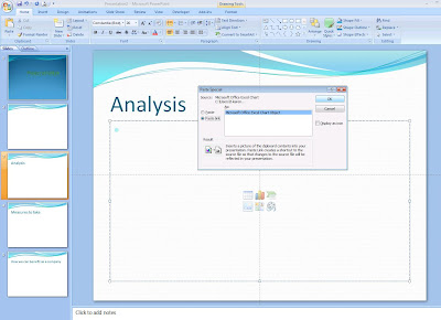
After this, just specify the area to place imported data, for this I am going to select the current sheet, just below my Total Sales value. You can choose your own settings for the imported data, to do this click on the Properties button.

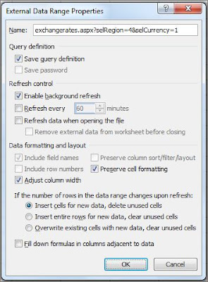
You will see a window like this where you can select the suitable 'Refresh Control' (for instance) for that data that you're importing from the web. Everytime the data changes in the browser, it will be reflected in your excel sheet.



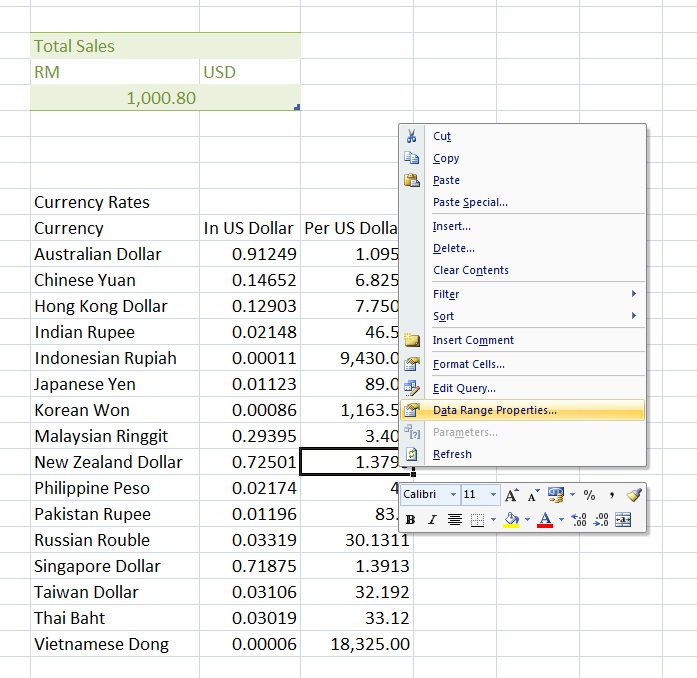
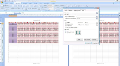
Click 'Ok' and you will have the same currency rates table placed in your excel sheet at the location that you have specified. Here I have right-clicked and when you choose the 'Data Range Properties' you will see the same settings when you hit the 'Properties' button previously. 'Refresh' there indicates that the data is live/linked to the web.

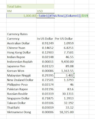
I shall refer to the value here and use it in my conversion formula and not have worries of inaccuracy or doing repeatitive formula updates.

Oh yea.... CHEERS to an exciting 2010 for all.... especially with the launch of Office 2010 coming soon :)

Bubbles in Excel chart

How you ever created a bubble chart in Excel? I reckon that most of us stick to the usual bar and pie chart and the occasional line chart. Right now, I'm going to show you how to create a 3D bubble chart to represent your data.

The information in my excel here is about the market share of numerous browsers for March 2009 which I obtained from Market Share site.

First of all, let me format the data block into a table to ease the process of adding columns, rows and formula.

I have just added another column for the existence duration of each browser respectively. Formula used is 2009 - (Start Year), simple right.

I have moved the columns around a bit so that I can get the exact visualization for my bubble chart. Ok, the most obvious difference of the bubble chart compared to the rest is that it needs 3 parameters - x, y, and z value which need to have numerical value. Right now, x-axis is the Start Year (Release Year) of the browser, y-axis is the percentage of Market Share (March 2009) for the browser and z value would be represented by the size of the bubble which in my chart reflects the duration or how long the browser has been in the market. So that's regarding understanding and positioning your data.

Let's start creating the chart, select the data for column 2 till column 4 (Start Year, Total Market Share, Duration), then click on the Insert tab, and in the Charts group, choose 'Other Charts', in the drop down, you will see 'Bubble with a 3-D effect', alternatively you could use the Office 2007 shortcut keys - simply type Alt (to see the shourtcut keys) - N (Insert tab) - O (Other Charts)


There you go, your very own Bubble chart.

My work's not done yet, for I'm not too satisfied with how it looks. I want each bubble to represent each browser and have it's own significant colour. When the chart is generated automatically (remember earlier I mentioned that x,y,and z has to have numerical value) very minimal 'personalization' so to speak was done to the values.

Let's make our chart look better, look at the ribbon, the contextual tab for Chart Tools has appeared and in the Design tab, click on Select Data.


In the dialog box, what we need to do is to edit the Series.

Choose the appropriate values for the Series Name, x, y and z value.

So for the first bubble, the values should look like this, I have highlighted the data row for the bubble.

Next, 'Add' the Series and do the same thing for all the browsers' information.

Finally, the 'Select Data' dialog box would have all the browser names enlisted in the Legend Entries area.

Do you like what you see... I know I do :)

Pasting Link?

I like this feature a lot. Here is a spreadsheet with figures and also a bar chart of the figures, which in this case is the yearly expenditure for printing in the company.

Now, assuming that I have a presentation to deliver, and I need this chart to be in one of the slides, I would typically, copy the slide (right-click + copy or Ctrl + C)

Ok my presentation deck is as shown, and I would like to place my copied chart in the Analysis slide here. I click on 'Paste' (Home tab) and choose 'Paste Special'. The dialog box opens, and I choose to Paste Link, the screen tip explains that Paste Link creates a shortcut to the source file so that any changes that occur will be reflected in the slide. Your chart is now in the slide you selected.

Back to the source file, let's check whether changes will be automated or not. I have just ammended the value for 2008, from '5605' to '7005'.


In powerpoint, right-click the chart, and choose to 'Update Link' and the change is reflected! Therefore if you have correctly pasted link for your charts, etc, when the values in the source file changes, these charts in your powerpoint slides will be updated when you open your deck.

Let me continue with my presentation slides. This presentation is about encouraging the company to 'Go Green', so right now I would like to visualize how one of the business processes is being done currently, and unfortunately it utilizes high amount of paper.

I remember seeing a diagram in an existing slide, so instead of redrawing it with shapes, text boxes, and icons, all I need to do is go to the Home tab, click on New Slide, and opt for the 'Reuse Slide' button.

A side pane will appear on the right, and here I will specify the path of the deck in which the diagram could be found by clicking on Browse > Browse File.

When you hover over the slides, you get a magnified view of it, and by clicking on it, the slides gets inserted into you current set of slides - much easier and faster than copy + paste right :)

Before you print your excel sheet

I got this question from a session I recently conducted, about a few things that can be done to your excel sheet just before you click on that 'Print' button.

My excel sheet here is a lengthy one, horizontally.

When I press on the 'Ctrl + End' buttons to show the last cell, see how far my data is stretched across.

Before anything, allow me to make my data look much more interesting, here I have formatted them into a table, and chosen a girly pink theme to it :)

My columns are consuming too much space, let me do 'Auto-fit' quickly. Select the whole table by just clicking on the tiny diagonal arrow at the top left corner, then double-click on any one of the columns' borders.

To have a look at how the document will look like after printing, we could go to Print Preview or from the View tab, click on Page Layout for the whole overall view of the pages.

My table's first row of columns contain the year, and I want this to be repeated on all the printed page, but first so that it's easier for you to notice, I have right-clicked and chosen Format Cells to put in a purple fill into the cells.

Here is how it is now from the Page Layout View.

Right now, click on the Page Layout tab, and the Page Setup group label, click on Print Titles. In the 'Print Titles' category of the dialog box, there is a portion for 'Columns to repeat at the left:', click into the text box there and select the left-most column of the table; '$A:$A' will be the value in the text box.

Now see the outcome from Page Layout View.

Sometimes you may want to adjust the Page Breaks in the excel sheet so that you can determine/control what is to be printed in one page, well, let's click on the Office Button and choose Excel Options. In the Advanced tab, check this capability:

Having done so, click on the View tab, and choose Page Break Preview.

You may now click on the intended Page Break and drag it to your point of choice. Another way to insert a Page Break would be to select the column and right-click, and select 'Insert Page Break'.

The conventional way of doing the Page Break is from the Page Layout tab, in the Page Setup group, there is button for Breaks, click on it and you will see options to 'Insert', 'Remove' or to 'Reset' page breaks.


Afterthis, please remember the environment when you do you printing, that means, make sure you have done all your editing and is pleased with the Print Preview or the Page Layout View before you decide to go ahead with the printer.

Hide and Seek with Excel

Sometimes when I work in Excel, I have some formulas which I want to keep away from people viewing the document so that they don't accidentally or intentionally change the values. This protection is only on the cell level and not for the whole workbook.

This is my excel sheet with a simple table that calculates the interest based on the principal, rate, and duration. I have clicked on the highlighted cell so that you can have a look at my formula.

First, we should set the protection for the cell, select the range of cells and right-click. Select Format Cell.
In the Protection tab, check Lock and Hidden.

From the ribbon, click on the Review tab, and in the Changes group, select 'Protect Sheet' so that cell range we selected just now will be locked and the formula hidden. You can also specify a password here, but I have chosen not to for this example.

Now when I click on the highlighted cell, the formula is not visible.

Here's what happened when I tried to edit the cell :

To remove the protection, just turn it off by clicking on 'Unprotect Sheet'. If a password was specified initially, then there will be a prompt first before the protection is turned off.

Next time you have cells with sensitive values or formulas, protect the values by locking and hiding the values.